Announcing nationalparkscolors - Color palettes inspired by America's National Parks

Bring the beauty of the great outdoors to your data visualizations

By Kailas Venkitasubramanian in R package Data Science

February 15, 2026

“In every walk with nature, one receives far more than he seeks.” - John Muir

I’m excited to announce nationalparkscolors, an R package that brings the beauty of America’s National Parks to your data visualizations. The package provides 20 carefully crafted color palettes, each inspired by the natural landscapes, geology, and ecosystems of some of the most iconic parks in the country.

The Inspiration

Anyone who has visited a National Park knows the feeling – the colors of nature are striking, harmonious, and deeply memorable. The golden bacterial mats of Yellowstone’s hot springs, the layered reds and ochres of the Grand Canyon, the deep glacial blue of Crater Lake – these are colors that tell a story.

I wanted to capture that feeling in a tool that data scientists and R users could reach for every day. Each palette in this package was designed with attention to:

Natural authenticity: Colors are drawn directly from the geology, flora, water, and sky of each park
Color harmony: Palettes use complementary, analogous, or triadic color relationships
Perceptual uniformity: Colors are distinguishable and accessible
Data visualization best practices: Palettes work for both categorical (discrete) and continuous data

This package is inspired by the excellent Wes Anderson Palettes package by Karthik Ram.

Installation

# install.packages("devtools")
devtools::install_github("kvenkita/nationalparkscolors")

library(nationalparkscolors)

# See all available palettes
names(natparks_palettes)
#>  [1] "Yellowstone"   "GrandCanyon"   "Yosemite"      "Zion"         
#>  [5] "Acadia"        "RockyMountain" "Smokies"       "Glacier"      
#>  [9] "Olympic"       "Arches"        "JoshuaTree"    "Everglades"   
#> [13] "BryceCanyon"   "GrandTeton"    "Shenandoah"    "Denali"       
#> [17] "Sequoia"       "CraterLake"    "DeathValley"   "Badlands"

The Palettes

The package includes 20 palettes spanning parks from coast to coast. Hover over any color to see its hex code.

Yellowstone National Park

Golden bacterial mats, deep blue pools, orange-brown bison, grey-white steam, and evergreen forests

#F4E04D

#4A90E2

#D97826

#8B7D6B

#2C5F2D

natparks_palette("Yellowstone")

Grand Canyon National Park

Red rock layers, terracotta cliffs, sandy beige formations, dusty rose, and deep canyon shadows

#C1440E

#D4704B

#E8B88A

#B8917A

#4A3728

natparks_palette("GrandCanyon")

Yosemite National Park

Granite grey of Half Dome, waterfall mist blue, meadow greens, deep pine, and sunset glow on El Capitan

#8B9A9D

#B8D4E0

#7CA860

#3D5941

#F0C987

natparks_palette("Yosemite")

Zion National Park

Navajo sandstone red, canyon shadows, river blue-green, desert sage, and burnt sienna

#D84A3B

#6B4E3D

#5C9EAD

#9FA674

#A0522D

natparks_palette("Zion")

Acadia National Park

Atlantic ocean blue, coastal granite grey, pink granite, forest green, and lighthouse white

#2E5266

#6E8898

#D49A9A

#4A7C59

#E8DCC4

natparks_palette("Acadia")

Glacier National Park

Glacial turquoise lakes, mountain grey, wildflower magenta, rocky brown, and dense forest green

#4DA6B3

#8B8D8E

#D64E93

#846658

#3B5441

natparks_palette("Glacier")

Great Smoky Mountains National Park

Blue mountain mist, forest green, rhododendron pink, autumn orange, and deep forest shadows

#748B9E

#5F7C5D

#E8A0BF

#D4824B

#2F3E2E

natparks_palette("Smokies")

Crater Lake National Park

Deep crater lake blue, caldera rim grey, sky reflection, volcanic rock, and pristine snow

#003F87

#6B7C8C

#87B5D6

#54555A

#E8F0F5

natparks_palette("CraterLake")

Bryce Canyon National Park

Orange-red hoodoos, pink limestone, cream formations, iron-stained red, and shadow purple

#E87451

#F4A6A3

#F8E5D0

#B8634F

#8B6F8B

natparks_palette("BryceCanyon")

Death Valley National Park

White salt flats, Artist's Palette pink, desert gold, volcanic black rocks, and oxidized green minerals

#F4F1E8

#E8A4B8

#D4A449

#3A3A3A

#8B9B76

natparks_palette("DeathValley")

And 10 more: RockyMountain, Olympic, Arches, JoshuaTree, Everglades, GrandTeton, Shenandoah, Denali, Sequoia, and Badlands. See the full list with names(natparks_palettes).

Using with ggplot2

Here are examples showing how to use these palettes in real visualizations.

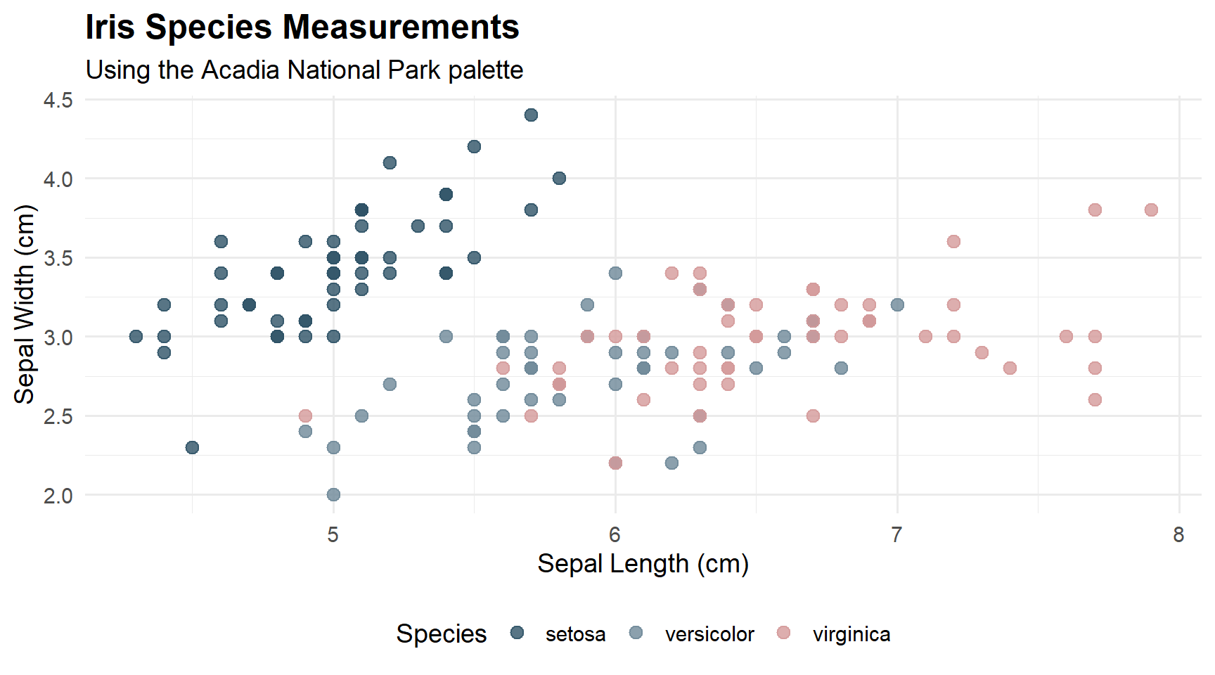
Scatter Plot – Acadia Palette

library(ggplot2)

ggplot(iris, aes(x = Sepal.Length, y = Sepal.Width, color = Species)) +
  geom_point(size = 3, alpha = 0.8) +
  scale_color_manual(values = natparks_palette("Acadia")) +
  labs(
    title = "Iris Species Measurements",
    subtitle = "Using the Acadia National Park palette",
    x = "Sepal Length (cm)",
    y = "Sepal Width (cm)"
  ) +
  theme_minimal(base_size = 14) +
  theme(
    plot.title = element_text(face = "bold", size = 18),
    legend.position = "bottom"
  )

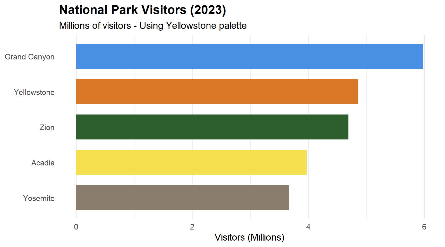
Bar Chart – Yellowstone Palette

park_visitors <- data.frame(
  Park = c("Yellowstone", "Grand Canyon", "Yosemite", "Zion", "Acadia"),
  Visitors = c(4.86, 5.97, 3.67, 4.69, 3.97),
  stringsAsFactors = FALSE
)

ggplot(park_visitors, aes(x = reorder(Park, Visitors), y = Visitors, fill = Park)) +
  geom_col(show.legend = FALSE, width = 0.7) +
  scale_fill_manual(values = natparks_palette("Yellowstone")) +
  coord_flip() +
  labs(
    title = "National Park Visitors (2023)",
    subtitle = "Millions of visitors - Using Yellowstone palette",
    x = NULL,
    y = "Visitors (Millions)"
  ) +
  theme_minimal(base_size = 14) +
  theme(
    plot.title = element_text(face = "bold", size = 18),
    panel.grid.major.y = element_blank()
  )

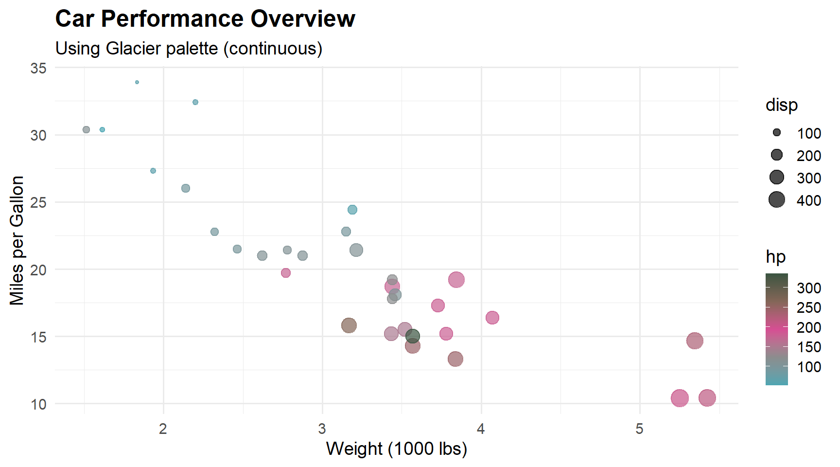
Continuous Scale – Glacier Palette

ggplot(mtcars, aes(x = wt, y = mpg, color = hp, size = disp)) +
  geom_point(alpha = 0.7) +
  scale_color_gradientn(colors = natparks_palette("Glacier", type = "continuous")) +
  labs(
    title = "Car Performance Overview",
    subtitle = "Using Glacier palette (continuous)",
    x = "Weight (1000 lbs)",
    y = "Miles per Gallon"
  ) +
  theme_minimal(base_size = 14) +
  theme(plot.title = element_text(face = "bold", size = 18))

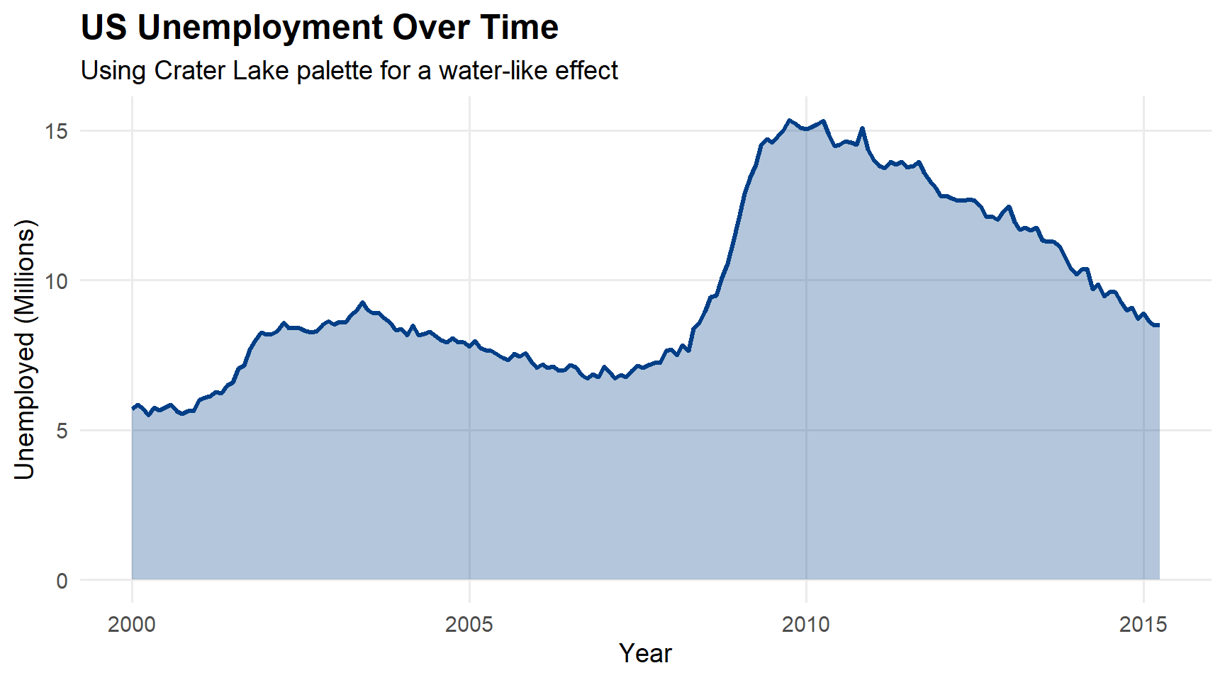
Time Series – Crater Lake Palette

library(dplyr)

economics_subset <- economics %>%
  filter(date >= as.Date("2000-01-01"))

ggplot(economics_subset, aes(x = date, y = unemploy / 1000)) +
  geom_line(color = natparks_palette("CraterLake")[1], linewidth = 1.2) +
  geom_area(fill = natparks_palette("CraterLake")[1], alpha = 0.3) +
  labs(
    title = "US Unemployment Over Time",
    subtitle = "Using Crater Lake palette for a water-like effect",
    x = "Year",
    y = "Unemployed (Millions)"
  ) +
  theme_minimal(base_size = 14) +
  theme(
    plot.title = element_text(face = "bold", size = 18),
    panel.grid.minor = element_blank()
  )

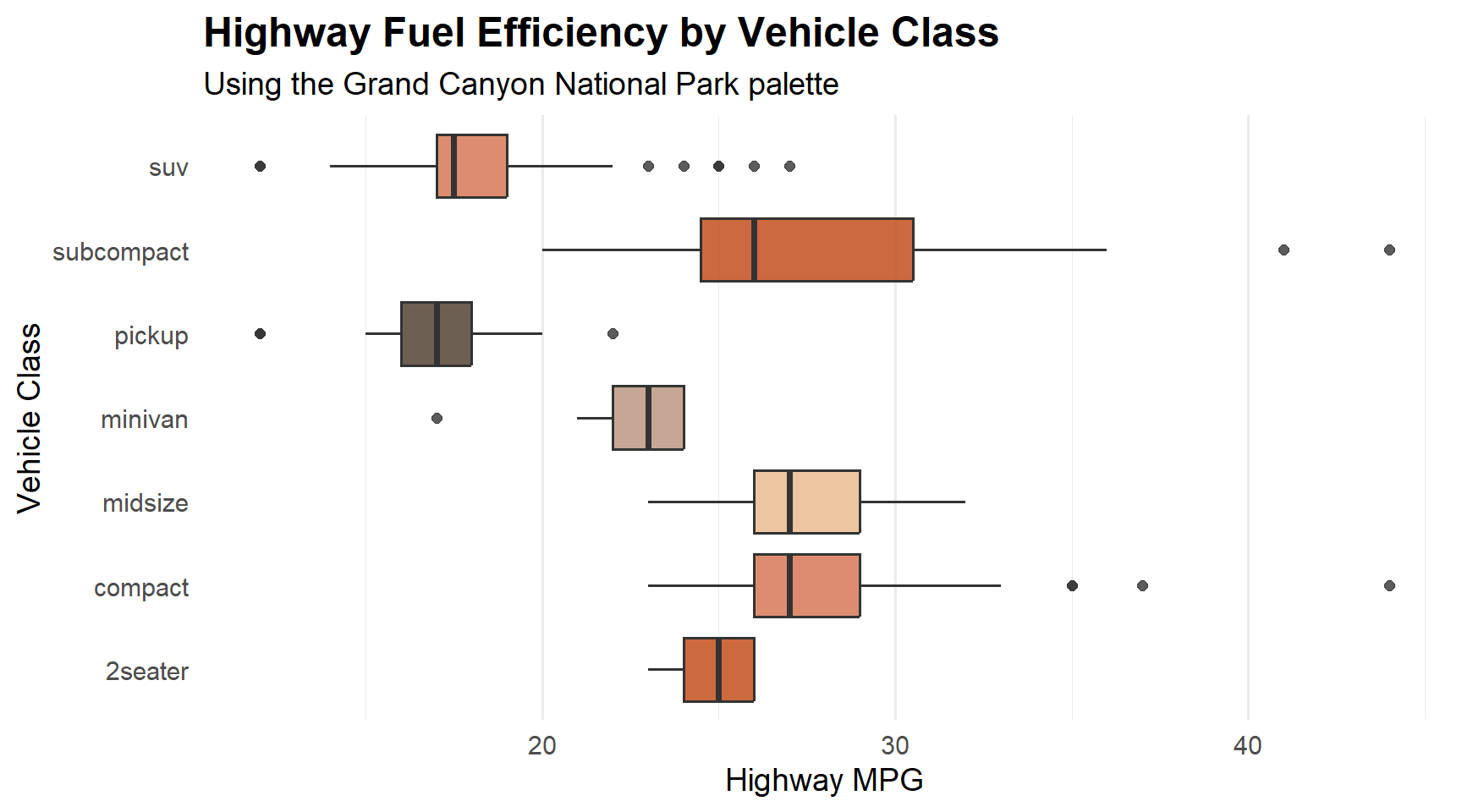
Box Plot – Grand Canyon Palette

ggplot(mpg, aes(x = class, y = hwy, fill = class)) +
  geom_boxplot(show.legend = FALSE, alpha = 0.8) +
  scale_fill_manual(values = rep(natparks_palette("GrandCanyon"), 2)) +
  coord_flip() +
  labs(
    title = "Highway Fuel Efficiency by Vehicle Class",
    subtitle = "Using the Grand Canyon National Park palette",
    x = "Vehicle Class",
    y = "Highway MPG"
  ) +
  theme_minimal(base_size = 14) +
  theme(
    plot.title = element_text(face = "bold", size = 18),
    panel.grid.major.y = element_blank()
  )

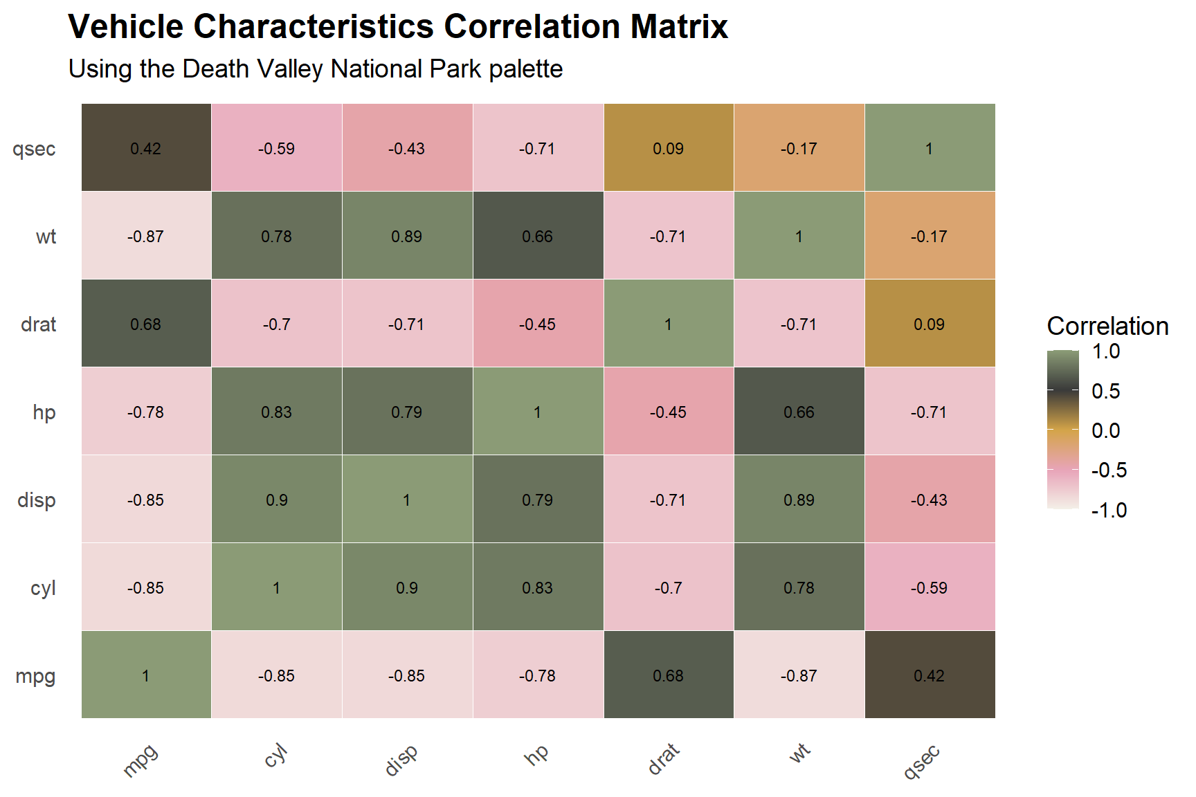
Heatmap – Death Valley Palette

mtcars_cor <- cor(mtcars[, 1:7])
mtcars_cor_df <- as.data.frame(as.table(mtcars_cor))
names(mtcars_cor_df) <- c("Var1", "Var2", "Correlation")

ggplot(mtcars_cor_df, aes(x = Var1, y = Var2, fill = Correlation)) +
  geom_tile(color = "white") +
  scale_fill_gradientn(
    colors = natparks_palette("DeathValley", 100, type = "continuous"),
    limits = c(-1, 1)
  ) +
  geom_text(aes(label = round(Correlation, 2)), size = 3) +
  labs(
    title = "Vehicle Characteristics Correlation Matrix",
    subtitle = "Using the Death Valley National Park palette",
    x = NULL, y = NULL
  ) +
  theme_minimal(base_size = 14) +
  theme(
    plot.title = element_text(face = "bold", size = 18),
    axis.text.x = element_text(angle = 45, hjust = 1),
    panel.grid = element_blank()
  )

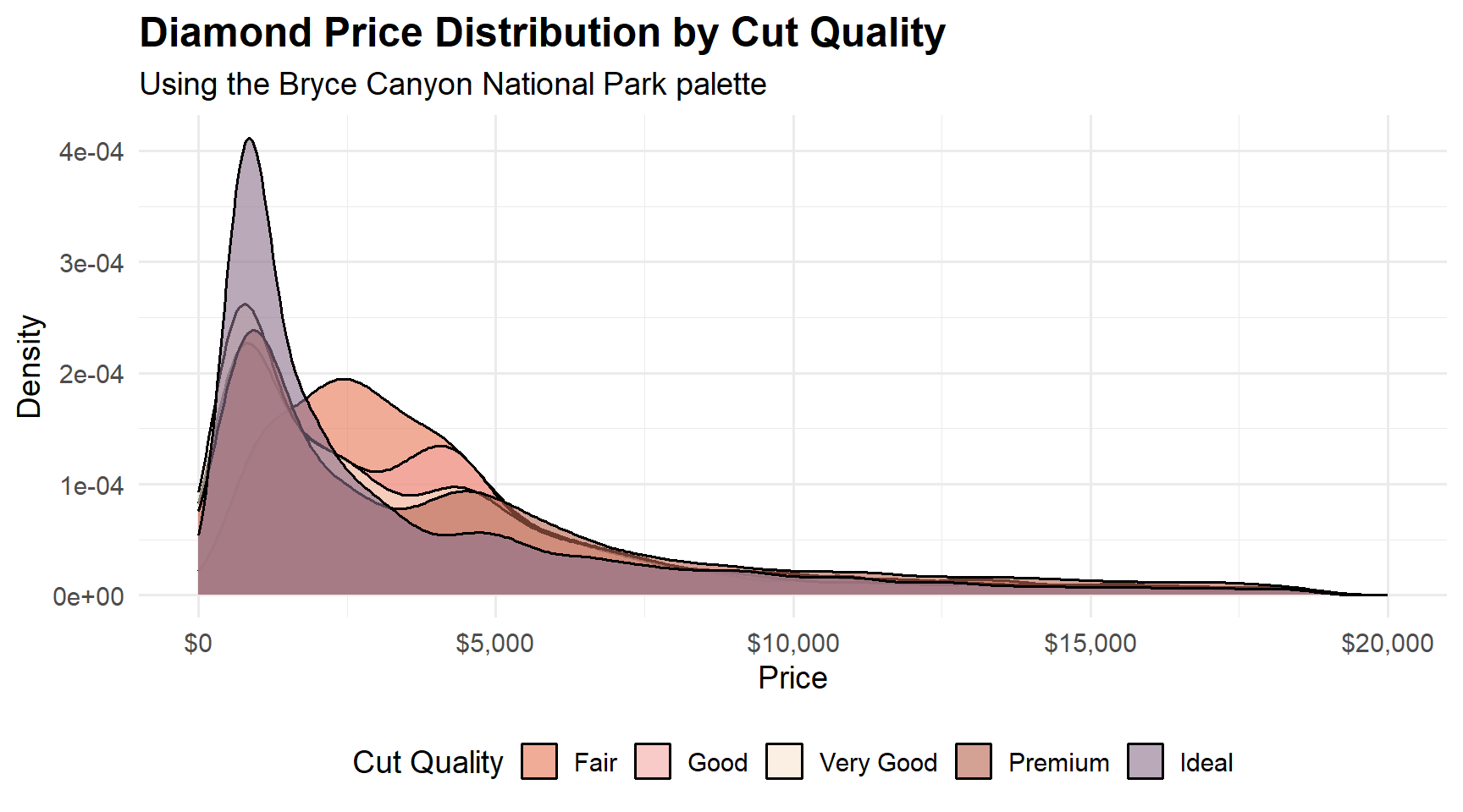
Density Plot – Bryce Canyon Palette

ggplot(diamonds, aes(x = price, fill = cut)) +
  geom_density(alpha = 0.6) +
  scale_fill_manual(values = natparks_palette("BryceCanyon")) +
  scale_x_continuous(labels = scales::dollar_format(), limits = c(0, 20000)) +
  labs(
    title = "Diamond Price Distribution by Cut Quality",
    subtitle = "Using the Bryce Canyon National Park palette",
    x = "Price",
    y = "Density",
    fill = "Cut Quality"
  ) +
  theme_minimal(base_size = 14) +
  theme(
    plot.title = element_text(face = "bold", size = 18),
    legend.position = "bottom"
  )

Palette Selection Guide

Use Case	Recommended Palettes
Categorical data (3-5 groups)	Use any discrete palette as-is
Continuous / gradient data	Add `type = "continuous"` to interpolate
Diverging data	Palettes with warm-to-cool transitions (Zion, Glacier)
Maps and choropleth	Single-hue gradients (CraterLake, RockyMountain)
Time series	Calm, flowing colors (CraterLake, Olympic)
Warm / earth tones	GrandCanyon, Arches, Yellowstone, BryceCanyon
Cool / water tones	CraterLake, Acadia, Glacier, Olympic